Back in 2022 I worked on a project with an ESP32 board with two sensors - an OV2640 optical camera and an MLX90640 low-resolution thermal sensor. The camera will give an MJPEG stream, and the thermal sensor returned a 32 x 24 array of temperatures on every HTTP request. On the server side, a Python app read the stream with OpenCV, ran a TensorFlow Lite object detection model on each frame, and showed the result in a small Flask UI. See the YouTube video i uploaded
The goal was to detect the trained object and sense its temperature. We initially had to train the target object, I started with a glass of hot water.
The model gives a bounding box in pixel coordinates on a 1024 x 768 frame (because with the camera - it is what is sees). But the temperature it detected is in a 32 x 24 grid coordinate space. So the real problem was this: if the object is at a certain point in the camera frame, which cell in the thermal grid is that same spot?
There are two reasons this needed solving. First, each sensor only does half the job. The camera can recognise the glass but can’t measure heat. The thermal sensor measures heat but, at 32 x 24, can’t recognise anything. So we need both. Second, they see the same scene at different resolutions, so the same spot has different coordinates in each. In the camera it might be (590, 482), and in the thermal grid it’s (18, 15). If both had the same resolution and were perfectly aligned, there would be nothing to convert. They don’t, so we need a way to translate one into the other.
The answer turned out to be simple arithmetic. But it only clicked once I understood something I honestly did not know at the time: an image is just an array of numbers. So let’s start there, slowly.
An image is a NumPy array
I was reading frames from the camera stream with OpenCV. When you call cap.read(), you don’t get back some special “image” object. You get a NumPy ndarray.
success, frame = cap.read()
print(frame.shape)   # (768, 1024, 3)
print(frame.dtype)   # uint8
That shape tells you everything. The frame is 768 rows tall and 1024 columns wide. Each element at a row and column is a pixel. Each pixel holds 3 values, one per colour channel. OpenCV stores them in BGR order (blue, green, red), not RGB. The dtype is uint8, so every value is an integer from 0 to 255.
If you print a small slice of the array, it looks like this:
row 0:  [12, 40, 200]  [13, 41, 198]  [15, 44, 190] ...
row 1:  [11, 39, 201]  [14, 42, 196]  [16, 45, 188] ...
row 2:  ...
That’s the whole image. Rows and columns of numbers.
  flowchart LR
    A[Camera stream] --> B["OpenCV cap.read()"]
    B --> C["NumPy ndarray<br/>shape (768, 1024, 3)<br/>uint8, BGR"]
Once this clicked for me, a lot of things got simpler. If an image is an array, then a position in the image is just an index: a row and a column. And you can do plain arithmetic on indexes.
The thermal sensor is also an array
So the camera side is just an array. That’s half the setup. The other half is the thermal sensor, and that’s where the temperatures come from. It gave me data in a much rawer form. Every request returned one long comma-separated string of 768 values. Each value was a temperature reading.
A flat list of 768 numbers doesn’t mean much on its own. But the sensor sees the scene as a grid of 24 rows and 32 columns, and 24 x 32 is exactly 768. So I parsed the string and reshaped it into a 2D array:
temps = np.array([float(v) for v in raw.split(",")])   # shape (768,)
grid = temps.reshape(24, 32)                            # shape (24, 32)
reshape doesn’t change the data. It just tells NumPy how to read the same 768 numbers: fill row 0 with the first 32 values, row 1 with the next 32, and so on. This is called row-major order.
Now the thermal data looks just like the camera frame. Rows and columns. The only difference is that each cell holds one float (a temperature) instead of three colour channels.
row 0:  [24.1, 24.3, 24.0, 25.2, ...]
row 1:  [24.0, 24.4, 26.8, 31.5, ...]
row 2:  ...
So now I had two arrays describing the same scene.
  flowchart LR
    S[Same scene] --> C[Optical camera]
    S --> H[Thermal sensor]
    C --> G1["frame<br/>(768, 1024, 3)<br/>colour"]
    H --> G2["grid<br/>(24, 32)<br/>temperature"]
Two arrays, very different resolutions
Having both sensors as arrays is nice, but it doesn’t solve anything yet. Here is the catch: they are nowhere near the same size. The camera frame is high resolution. The thermal grid is tiny. And that size gap is exactly why we need two sensors in the first place.
The camera is great for figuring out what is in the scene, and that’s what the object detection model needs. But it knows nothing about heat. The thermal sensor knows how hot each part of the scene is, but at 32 x 24 an object is just a warm blob. You can’t detect anything in it.
So each sensor had half the answer. The camera could tell me where the object was. The thermal sensor could tell me how hot things were. I needed a way to join the two.
To join them, I had to understand how the two arrays line up. Compare the resolutions:
- Width: 1024 pixels vs 32 cells. 1024 ÷ 32 = 32
- Height: 768 pixels vs 24 cells. 768 ÷ 24 = 32
Same number on both axes. That’s the scale factor, and it means the two arrays have the same aspect ratio (4:3). Every thermal cell covers a 32 x 32 block of camera pixels. If you laid the small grid on top of the big one, each thermal cell would sit over 1,024 camera pixels.
  flowchart LR
    A["32 x 32 block<br/>of camera pixels<br/>(1,024 pixels)"] -->|"maps to"| B["1 thermal cell<br/>(1 temperature)"]
This is the key idea of the whole thing. To go from a camera coordinate to a thermal coordinate, divide by 32.
Plotting it on X and Y
So we know the rule: divide by 32. But divide what? We need a point in the camera frame that says “the object is here”. That point comes from the object detection model. Before we get it, it helps to picture both arrays as XY planes.
One thing that trips people up: image coordinates don’t work like the graphs from school. The origin (0, 0) is the top-left corner. X grows to the right. Y grows downward. In array terms, x is the column index and y is the row index.
When the detection model finds an object, it returns a bounding box. That’s just two corners in pixel coordinates, top-left and bottom-right. Here is a real one from the project, plotted on the camera’s 1024 x 768 plane:
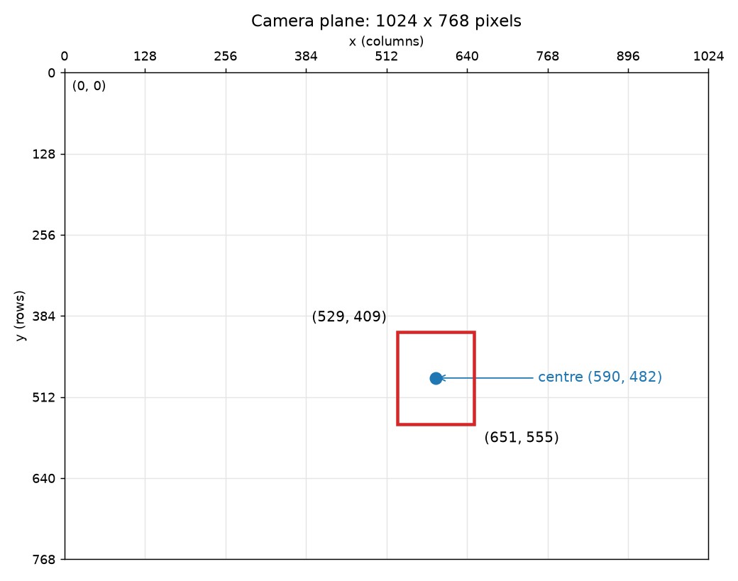
The centre point of the box, marked ●, is just the average of the two corners:
x = (529 + 651) // 2 = 590
y = (409 + 555) // 2 = 482
So the object is at (590, 482) on the camera plane. Now we need the same point on the thermal plane.
Shrink the point, not the image
At this point we have two things: a point on the camera plane, (590, 482), and the scale factor between the two planes, 32. The question is which side to change to make them meet.
My first instinct was that I’d have to resize something. Maybe upscale the thermal grid to 1024 x 768 so it matched the camera frame. But that wouldn’t give me any new information. The sensor only measured 768 temperatures. Upscaling would just fill in made-up values between the real readings.
The better move was the other way round. I didn’t need to resize either array. I only needed to scale the coordinates down. Just divide by the scale factor and drop the decimals. In Python that’s floor division, //:
x = 590 // 32 = 18
y = 482 // 32 = 15
So the camera point (590, 482) lands on thermal cell (18, 15). Here it is on the 32 x 24 plane. I’ve also scaled the box corners the same way, (16, 12) to (20, 17), so you can see where the object sits:
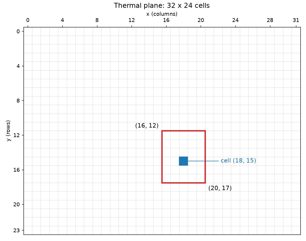
Each small square is one temperature reading. The box that covered thousands of pixels on the camera plane now covers a handful of cells.
The last step is to read that cell. One thing to watch: NumPy indexes as [row, column], which is [y, x]. So y comes first.
temperature = grid[15, 18] # row 15, column 18
That’s the object’s temperature.
  flowchart TD
    A["Camera frame<br/>1024 x 768"] --> B[Object detection]
    B --> C["Bounding box<br/>(529, 409) to (651, 555)"]
    C --> D["Centre point<br/>(590, 482)"]
    D --> E["Floor divide by 32<br/>(18, 15)"]
    E --> F["grid[15, 18]"]
    F --> G[Temperature]
The whole trick is a division. No image resizing, no extra library. Once I saw both sensors as arrays, the problem turned into “which cell in the small array sits under this point in the big one?” And that has a very simple answer.
Is this interpolation?
That covers the core idea. Now a small detour, because the word I used for all this back then was wrong. For a long time I called this step “interpolation”. It isn’t, and the difference is worth knowing.
Interpolation means estimating new values between the values you already have. Say you have temperature readings at cell 3 and cell 4, and you want a value at 3.5. Interpolation guesses one, usually as a weighted average of the neighbours. That’s what happens when you upscale an image: the new pixels have to come from somewhere, so they are interpolated. Bilinear and bicubic are common methods.
What I did is different. I never created any new values. I took a coordinate from a high-resolution space and mapped it into a low-resolution space with a scale factor. That’s downscaling the coordinates, or more plainly, coordinate mapping. Because floor division snaps every pixel to whichever cell it falls in, it behaves like nearest-neighbour sampling.
Interpolation did show up in the project, though, just not where I thought. When you plot a 32 x 24 grid on a screen, it gets stretched to hundreds of pixels wide. The plotting tool fills the gaps by interpolating, and that’s why a grid of only 768 readings can look smooth:
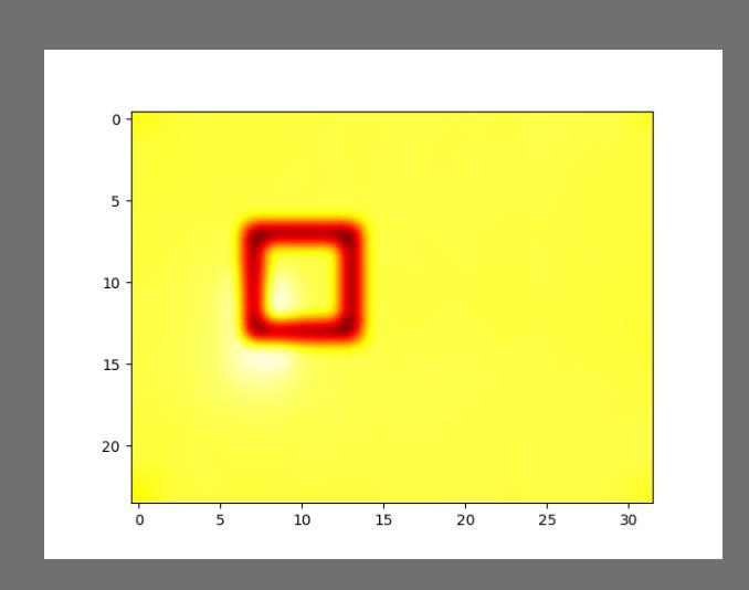
Look at the axes: 0 to 31 across, 0 to 23 down. That’s the thermal grid, with a scaled-down box drawn onto it (from a different frame than the example above). There are only 768 real values in that picture. Everything smooth between them is interpolation from the plotting step.
What about other objects in the scene?
Back to the mapping. One question I had to answer for myself: does the thermal sensor only return the temperature inside the bounding box?
No. The sensor knows nothing about bounding boxes. On every request it sends all 768 readings, one per cell, covering everything in its view. The glass, the table, the wall, and any other object that happens to be there.
The bounding box is what decides which of those 768 readings we use. That’s the whole point of the mapping. The model says “the glass is here” in camera coordinates, we convert that to a cell, and we read only that cell. Every other cell is ignored.
So if there’s a second object in the scene, its heat is in the grid too, just in different cells. We never read them, because the model was trained on the glass and only draws a box around the glass. In my setup I also limited the model to one detection at a time (the highest-scoring one), with a minimum confidence score of 0.4.
That’s how we know which object a temperature belongs to: we picked the cell from the glass’s own box. But it can still go wrong in a few ways:
- Objects right next to each other. Each thermal cell covers a 32 x 32 block of camera pixels. If another object sits right beside the glass, one cell can contain a bit of both, and the reading becomes a mix. This gets worse if it’s another glass of the same kind. Reading the centre of the box helps, since the centre is the cell most likely to be all glass.
- A wrong detection. If the model mistakes another object for the glass, we read the wrong temperature with full confidence. The score threshold is the guard here.
- The two sensors don’t line up. Even with a perfect detection, the cell we land on might actually be showing the object next to it. This one needs its own section.
Calibration: the two sensors aren’t in the same spot
So far, the divide-by-32 rule has quietly assumed something: that the camera and the thermal sensor see exactly the same view, with the same (0, 0) corner and the same area. In practice, they don’t.
The whole setup fits in a small box, roughly 8 x 5 cm. The camera sits at the top of the ESP32 board, and the thermal sensor is a separate part placed elsewhere in the box. So the two are looking at the scene from two slightly different spots, and possibly at slightly different angles. That’s enough for the glass to appear in a different place in each image. In the camera it might be dead centre. In the thermal grid it might be a few cells lower and off to one side.
So after dividing by 32, we land roughly on the right cell, but not exactly. And that’s dangerous in exactly the case from the last section: with two glasses side by side, a perfect detection could still send us to the cell that is actually showing the other glass.
Calibration means measuring that offset once and correcting for it every time. In my code it was just two numbers in a config file, tuned by hand:
YSHIFT = 3   # rows
XSHIFT = 1   # columns

temperature = grid[y + YSHIFT, x - XSHIFT]
After the division, move 3 rows down and 1 column left, to where the glass really shows up in the thermal grid. For our example, that moves the reading from grid[15, 18] to grid[18, 17].
There was one more alignment fix. Both the camera frame and the thermal array were flipped horizontally (cv2.flip(..., 1)), so that left and right meant the same thing in both.
A fixed shift like this has two limits worth knowing:
- It’s only exact at one distance. The offset between two lenses changes as the object moves closer or further away. It’s the same thing your two eyes do: a finger close to your face looks very different to each eye, a tree far away barely does. Calibrate with the glass at one distance, and the shift drifts as it moves.
- It fixes position, not size. If the two sensors have different fields of view, the scene isn’t the same width in both. A shift alone won’t line them up across the whole frame.
So calibration reduces the risk of reading the neighbour, but doesn’t remove it. The practical safeguard is to keep objects at least a cell or two apart, which is about 32 to 64 camera pixels.
A limit the code couldn’t fix
The MLX90640 is a thermal sensor array, not a thermal camera. It gives you 768 temperature readings and nothing more. It sat in the same small box as the ESP32 and the OV2640, and over time the device heated itself up. For a sensor whose whole job is measuring heat, that’s a problem, and in the end it made the device ineffective.
No amount of coordinate mapping or calibration fixes that. The mapping can point at the right cell, but it can’t make the reading in that cell trustworthy. That part is a hardware problem.
Takeaway
If there’s one thing to take from this post, it’s that an image is just a NumPy array. Once you see it that way, everything else here follows.
A pixel is one element at a row and a column, so it has an x and a y. A group of pixels, like the area inside a bounding box, is just a range of rows and columns. In NumPy that’s a slice: frame[409:555, 529:651] gives you exactly the pixels inside our example box. And because positions are just numbers, you can do plain arithmetic on them. Scale them, shift them, map them from one array onto another. That’s all this whole post did.
This is also why the idea goes well beyond this project. Pretty much anything that works with images, from photo filters to models that recognise handwriting, starts from the same place: an array of numbers. A model never really “sees” a picture. It gets those numbers and learns patterns from groups of neighbouring pixels.
And it comes full circle. The object detection model in this project worked the same way. It took the camera frame in as an RGB array, and what it gave back, the bounding box, was just a set of coordinates in that same array. So the model and my mapping code were speaking the same language: rows, columns and numbers. The model worked out where the object was, and a bit of arithmetic carried that answer over to the thermal array. Which is exactly where this post started.